Advanced Machine Learning Classification

Optimization with Stochastic Gradient Descent Implementing RMSProp and Numpy

Alan Mössinger — follow

Alan Mössinger on LinkedIn: Advanced Machine Learning Classification with Algorithms and Numpy…Advanced Machine Learning Classification with Algorithms and Numpy. Enjoy full code in my portfolio.
www.linkedin.com

Inthis comprehensive exploration, we delve into the intricacies of the linear model classifier, an integral component in the world of machine learning, particularly for binary classification tasks. Our focus will be on optimizing this model using the stochastic gradient descent (SGD) method, a powerful and efficient optimization technique. Throughout this journey, we will exclusively utilize numpy, a robust library for numerical computation in Python, renowned for its efficiency and versatility. Additionally, we will harness the fundamental principles of mathematics, the universal language that underpins all scientific endeavors.

Understanding the Linear Model Classifier

The linear model classifier operates by making predictions based on a linear function of the input features. It computes a weighted sum of the input features and then applies a threshold to determine the class. Despite its apparent simplicity, the linear model classifier is a surprisingly potent tool in the machine learning arsenal. It not only serves as an excellent starting point for beginners but also forms the foundation upon which more complex algorithms are built.

Optimizing with Stochastic Gradient Descent

Optimization of the linear model classifier is crucial for enhancing its performance and accuracy. Stochastic Gradient Descent (SGD) emerges as a hero in this scenario. Unlike traditional gradient descent, which uses the entire dataset to update model parameters, SGD randomly selects a subset of data for each iteration. This approach significantly reduces computational burden and speeds up the convergence process, making it particularly beneficial for large datasets.

The Power of Numpy

Numpy, a cornerstone in the Python scientific computing stack, offers an array of functionalities for efficiently handling numerical operations. Its array object is a central data structure, and numpy provides tools for performing operations on these arrays with ease and speed. By leveraging numpy, we can implement the linear model classifier and SGD algorithm in a manner that is not only computationally efficient but also highly scalable.

Practical Implementation Steps

1.Data Preparation: Start by preparing your data. Ensure that it is clean and formatted correctly for use in a linear model classifier.

with open('train.npy', 'rb') as fin:
    X = np.load(fin)

with open('target.npy', 'rb') as fin:
    y = np.load(fin)

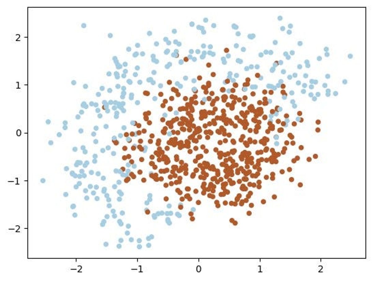
plt.scatter(X[:, 0], X[:, 1], c=y, cmap=plt.cm.Paired, s=20)
plt.show()

Raw data with clearly overlap

2. Model Construction: Construct the linear model classifier using numpy. Initialize the weights and bias terms.

def expand(X):
    """
    Adds quadratic features.
    This expansion allows your linear model to make non-linear separation.

    For each sample (row in matrix), compute an expanded row:
    [feature0, feature1, feature0^2, feature1^2, feature0*feature1, 1]

    :param X: matrix of features, shape [n_samples,2]
    :returns: expanded features of shape [n_samples,6]
    """

    X_expanded = np.zeros((X.shape[0], 6))
    '''This line initializes a new NumPy array X_expanded with the same number of
    rows as X but with 6 columns. It's filled with zeros to start with.'''

    X_expanded[:, 0] = X[:, 0]  # feature0
    X_expanded[:, 1] = X[:, 1]  # feature1
    '''These lines copy the original features from X into the first two columns of X_expanded.'''

    X_expanded[:, 2] = X[:, 0] ** 2  # feature0^2
    X_expanded[:, 3] = X[:, 1] ** 2  # feature1^2
    '''Here, the squares of each feature are calculated and stored in the third and fourth columns of X_expanded.'''

    X_expanded[:, 4] = X[:, 0] * X[:, 1]  # feature0 * feature1
    '''This line calculates the product of the two features (an interaction term) and stores it in the
    fifth column of X_expanded.'''

    X_expanded[:, 5] = 1  # constant term
    '''The sixth column of X_expanded is set to 1. This acts as a constant
    feature, which is useful for learning an intercept term in many linear models.'''

    return X_expanded


# Here are some tests for your implementation of expand function.

# Simple test on random numbers

dummy_X = np.array([
        [0,0],
        [1,0],
        [2.61,-1.28],
        [-0.59,2.1]
    ])

# call your expand function
dummy_expanded = expand(dummy_X)

# what it should have returned:   x0       x1       x0^2     x1^2     x0*x1    1
dummy_expanded_ans = np.array([[ 0.    ,  0.    ,  0.    ,  0.    ,  0.    ,  1.    ],
                               [ 1.    ,  0.    ,  1.    ,  0.    ,  0.    ,  1.    ],
                               [ 2.61  , -1.28  ,  6.8121,  1.6384, -3.3408,  1.    ],
                               [-0.59  ,  2.1   ,  0.3481,  4.41  , -1.239 ,  1.    ]])

3.SGD Optimization: Implement the SGD algorithm. This involves iteratively updating the model’s weights based on a subset of the data and the learning rate. We are applying RMSprop (Root Mean Square Propagation): This is an adaptive learning rate optimization algorithm designed to address some of the issues encountered with the stochastic gradient descent (SGD) method in training deep neural networks. RMSProp addresses the issue of a global learning rate by maintaining a moving average of the squares of gradients for each weight and dividing the learning rate by this average. This ensures that the learning rate is adapted for each weight in the model, allowing for more nuanced updtes.

RMSProp algorithm, which use squared gradients to adjust learning rate

4.Model Evaluation: Evaluate the model’s performance. You can use metrics such as accuracy, precision, recall, and the confusion matrix to assess how well your model performs.

Get Alan Mössinger’s stories in your inbox

Join Medium for free to get updates from this writer.

Subscribe

Since we train our model with gradient descent, we should compute gradients. To be specific, we need a derivative of loss function over each weight [6 of them].

Loss function

'''The function calculates the gradient of the loss function, which represents how much each element in the weight vector w needs to be adjusted to reduce the loss. This is essential for training the model to fit the data.
The function returns a vector (of the same length as the weight vector w) representing the gradient of the loss function. Each element of this
vector indicates the direction and magnitude of change needed for the corresponding weight to reduce the loss.
The gradient essentially tells us how much the loss would change if we changed each weight by a small amount. A positive gradient for a weight
suggests that increasing the weight will increase the loss, while a negative gradient suggests that increasing the weight will decrease the
loss. The optimizer uses this information to adjust the weights in a way that reduces the loss.'''

def compute_grad(X, y, w):
    '''Parameters:

    X: The feature matrix with a shape [n_samples, 6].
    y: The target vector of shape [n_samples]. It contains the actual class labels (1 or 0) for each sample.
    w: The weight vector of shape [6]'''

    """
    Given feature matrix X [n_samples,6], target vector [n_samples] of 1/0,
    and weight vector w [6], compute vector [6] of derivatives of L over each weights.
    Keep in mind that our loss is averaged over all samples (rows) in X.
    """

    '''probabilities = probability(X, w) calculates the predicted probabilities for each sample.
    grad = np.dot(X.T, (probabilities - y)) / num_samples computes the gradient. X.T is the transpose of X, which when
    multiplied by the difference (probabilities - y) and averaged over the number of samples, gives the gradient
    of the loss with respect to each weight.'''

    # Number of samples
    num_samples = X.shape[0]

    # Compute the predicted probabilities
    probabilities = probability(X, w)

    # Compute the gradient
    grad = np.dot(X.T, (probabilities - y)) / num_samples

    '''Number of Samples: The function first determines the number of samples (num_samples) in the dataset.
    Probability Calculation: It then calculates the predicted probabilities for each sample in X being in class 1, using the probability function and
    the current weights w.
    Computing the Gradient:
    The gradient of the loss function with respect to the weights is computed using the formula:
    grad = 1/ N ⋅ X⊤ ⋅ (p−y)
        Where:
            X⊤ is the transpose of the feature matrix X.
            p is the vector of predicted probabilities.
            y is the vector of actual labels.
            The product X⊤⋅(p−y) calculates the gradient for each weight.
            The result is then divided by the number of samples (num_samples) to average the gradient across all samples.'''


    return grad

5. Fine-Tuning: Experiment with different learning rates and iterations to fine-tune your model for optimal performance.

#Here's an auxiliary function that visualizes the optimal performance:

from IPython import display

h = 0.01
x_min, x_max = X[:, 0].min() - 1, X[:, 0].max() + 1
y_min, y_max = X[:, 1].min() - 1, X[:, 1].max() + 1
xx, yy = np.meshgrid(np.arange(x_min, x_max, h), np.arange(y_min, y_max, h))

def visualize(X, y, w, history):
    """draws classifier prediction with matplotlib magic"""
    Z = probability(expand(np.c_[xx.ravel(), yy.ravel()]), w)
    Z = Z.reshape(xx.shape)
    plt.subplot(1, 2, 1)
    plt.contourf(xx, yy, Z, alpha=0.8)
    plt.scatter(X[:, 0], X[:, 1], c=y, cmap=plt.cm.Paired)
    plt.xlim(xx.min(), xx.max())
    plt.ylim(yy.min(), yy.max())

    plt.subplot(1, 2, 2)
    plt.plot(history)
    plt.grid()
    ymin, ymax = plt.ylim()
    plt.ylim(0, ymax)
    display.clear_output(wait=True)
    plt.show()

Solution and convergence

FInal 2D — Decision Boundary Scatter Plot final results

# 3D-Plot and Video - Run this code in order to see a 3D animation

from mpl_toolkits.mplot3d import Axes3D

# Create a 3D figure
fig = plt.figure(figsize=(10, 8))
ax = fig.add_subplot(111, projection='3d')

# 3D scatter plot of the data points with actual labels
ax.scatter(X[:, 0], X[:, 1], y, c=y, cmap=plt.cm.Paired, s=20)

# Creating a meshgrid for the decision boundary
xx, yy = np.meshgrid(np.linspace(x_min, x_max, num=100), np.linspace(y_min, y_max, num=100))
Z = probability(expand(np.c_[xx.ravel(), yy.ravel()]), w)
Z = Z.reshape(xx.shape)

# Plot the decision boundary as a surface
ax.plot_surface(xx, yy, Z, rstride=1, cstride=1, alpha=0.3, cmap=plt.cm.coolwarm)

# Labels and title
ax.set_xlabel('Feature 0')
ax.set_ylabel('Feature 1')
ax.set_zlabel('Probability')
ax.set_title('3D Decision Boundary')

plt.show()

Press enter or click to view image in full size

3D — Decision Boundary final results

Conclusion:

The journey through understanding and optimizing a linear model classifier with SGD using numpy provides not just an insight into a fundamental machine learning technique but also a blueprint for approaching more complex models. This exploration underscores the importance of a solid foundation in basic algorithms and the power of efficient computational tools like numpy. As we dive deeper into these concepts, it becomes evident that such foundational knowledge and tools are indispensable in the vast and ever-evolving landscape of data science. Whether you’re a budding data scientist or a seasoned professional, mastering these core aspects paves the way for tackling more advanced challenges in the field, ultimately contributing to the exciting world of machine learning and data analysis.

Please follow me if the article was enjoyable.

I write about:

#Data Science, #AI, #Machine Learning, #Business Analytics, #Energy, #Project Management, #Strategy, #Decision-Making

You also can find me on:

Linedin

Github