Advanced Machine Learning

K-Nearest Neighbor: End-to-End Project and Full Python Code

Introduction

K-Nearest Neighbors is a supervised learning algorithm, where the data is ‘trained’ with data points corresponding to their classification. To predict the class of a given data point, it takes into account the classes of the ‘K’ nearest data points and chooses the class in which the majority of the ‘K’ nearest data points belong to as the predicted class.

The KNN algorithm calculates the probability of the test data belonging to the classes of ‘K’ training data and the class that holds the highest probability will be selected.

Then how to select the optimal K value?

There are no pre-defined statistical methods to find the most favorable value of K. Initialize a random K value and start computing. Choosing a small value of K leads to unstable decision boundaries. The substantial K value is better for classification as it leads to smoothening the decision boundaries. I have derive a plot between error rate and K denoting values in a defined range. Then we can choose the K value having a minimum error rate. Now you will get the idea of choosing the optimal K value by implementing the model. Enjoy the code!

Objectives

• Use K Nearest neighbors to classify data and find the optimal k-value and error

What is K-Nearest Neighbors?

The K-Nearest Neighbors algorithm is a type of supervised learning where the model is trained using data points along with their respective classifications. When predicting the class of a specific data point, it considers the classes of the ‘K’ closest data points. The predicted class is then determined by the majority class among these ‘K’ nearest data points.

The KNN algorithm calculates the probability of the test data belonging to the classes of ‘K’ training data and class holds the highest probability will be selected.

Here’s a nice visualization of the K-Nearest Neighbors algorithm.

Press enter or click to view image in full size

In this case, we have data points of Class A and B. We want to predict what the star (test data point) is. If we consider a k value of 3 (3 nearest data points), we will obtain a prediction of Class B. Yet if we consider a k value of 6, we will obtain a prediction of Class A.

In this sense, it is important to consider the value of k. Hopefully from this diagram, you should get a sense of what the K-Nearest Neighbors algorithm is. It considers the ‘K’ Nearest Neighbors (data points) when it predicts the classification of the test point.

Then how to select the optimal K value?

In the realm of machine learning, specifically when working with the K-Nearest Neighbors (KNN) algorithm, there are no universally accepted statistical methods to determine the most optimal value for ‘K’. The process typically begins by initializing a random value for ‘K’ and then proceeding with the computations.

The choice of ‘K’ is crucial as it can significantly impact the model’s performance. If a small value for ‘K’ is chosen, it can lead to unstable decision boundaries. This is because a small ‘K’ value means the algorithm heavily relies on the immediate neighbors, which can be influenced by noise in the data, leading to overfitting.

On the other hand, choosing a larger ‘K’ value tends to yield better results for classification tasks. This is because a larger ‘K’ value has the effect of smoothing the decision boundaries, reducing the impact of noise and outliers on the classification. However, if ‘K’ is too large, the model may become too generalized, leading to underfitting.

To find the optimal ‘K’ value, one common approach is to derive a plot between the error rate and ‘K’ values within a specified range. This plot is often referred to as an “elbow curve”. As ‘K’ increases, the error rate decreases until it reaches a point of minimum error — the ‘elbow’ of the curve. This ‘K’ value at the elbow point is typically chosen as the optimal ‘K’ value as it balances bias and variance, leading to a model that generalizes well to unseen data.

By implementing the model with this chosen ‘K’ value, you can gain a practical understanding of how to select the optimal ‘K’ value in the K-Nearest Neighbors algorithm. Remember, the optimal ‘K’ value may vary depending on the specific dataset and problem at hand, so it’s always a good idea to experiment with different ‘K’ values.

Calculating distance:

The first step is to calculate the distance between the new point and each training point. There are various methods for calculating this distance, of which the most commonly known methods are — Euclidian, Manhattan (for continuous) and Hamming distance (for categorical).

Euclidean Distance: Euclidean distance is calculated as the square root of the sum of the squared differences between a new point (x) and an existing point (y).

Manhattan Distance: This is the distance between real vectors using the sum of their absolute difference.

Table of contents

1. About the dataset
2. Data Visualization and Analysis
3. Classification

Let’s load required libraries

import numpy as np
import matplotlib.pyplot as plt
import pandas as pd
import numpy as np
from sklearn import preprocessing
%matplotlib inline

About the dataset

Imagine a telecommunications provider has segmented its customer base by service usage patterns, categorizing the customers into four groups. If demographic data can be used to predict group membership, the company can customize offers for individual prospective customers. It is a classification problem. That is, given the dataset, with predefined labels, we need to build a model to be used to predict class of a new or unknown case.

The example focuses on using demographic data, such as region, age, and marital, to predict usage patterns.

The target field, called custcat, has four possible values that correspond to the four customer groups, as follows: 1- Basic Service 2- E-Service 3- Plus Service 4- Total Service

Our objective is to build a classifier, to predict the class of unknown cases. We will use a specific type of classification called K nearest neighbour.

Load Data

Let’s read the data using pandas library and print the first five rows.

df = pd.read_csv('https://cf-courses-data.s3.us.cloud-object-storage.appdomain.cloud/IBMDeveloperSkillsNetwork-ML0101EN-SkillsNetwork/labs/Module%203/data/teleCust1000t.csv')
df.head()

region  tenure  age  marital  address  income  ed  employ  retire  gender  reside  custcat
0  2  13  44  1  9  64.0  4  5  0.0  0  2  1
1  3  11  33  1  7  136.0  5  5  0.0  0  6  4
2  3  68  52  1  24  116.0  1  29  0.0  1  2  3
3  2  33  33  0  12  33.0  2  0  0.0  1  1  1
4  2  23  30  1  9  30.0  1  2  0.0  0  4  3

Data Visualization and Analysis

Let’s see how many of each class is in our data set

df.info()


<class 'pandas.core.frame.DataFrame'>
RangeIndex: 1000 entries, 0 to 999
Data columns (total 12 columns):
 #   Column   Non-Null Count  Dtype
---  ------   --------------  -----
 0   region   1000 non-null   int64
 1   tenure   1000 non-null   int64
 2   age      1000 non-null   int64
 3   marital  1000 non-null   int64
 4   address  1000 non-null   int64
 5   income   1000 non-null   float64
 6   ed       1000 non-null   int64
 7   employ   1000 non-null   int64
 8   retire   1000 non-null   float64
 9   gender   1000 non-null   int64
 10  reside   1000 non-null   int64
 11  custcat  1000 non-null   int64
dtypes: float64(2), int64(10)
memory usage: 93.9 KB

Let’s see how many of each class is in our data set

df['custcat'].value_counts()



custcat
3    281
1    266
4    236
2    217
Name: count, dtype: int64

281 Plus Service, 266 Basic-service, 236 Total Service, and 217 E-Service customers

You can easily explore your data using visualization techniques:

df.hist(column='income', bins=50)

Feature set

Let’s define feature sets, X:

df.columns

Index(['region', 'tenure', 'age', 'marital', 'address', 'income', 'ed',
       'employ', 'retire', 'gender', 'reside', 'custcat'],
      dtype='object')

To use scikit-learn library, we have to convert the Pandas data frame to a Numpy array:

X = df[['region', 'tenure','age', 'marital', 'address', 'income', 'ed', 'employ','retire',
        'gender', 'reside']] .values  #.astype(float)
X[0:5]

array([[  2.,  13.,  44.,   1.,   9.,  64.,   4.,   5.,   0.,   0.,   2.],
       [  3.,  11.,  33.,   1.,   7., 136.,   5.,   5.,   0.,   0.,   6.],
       [  3.,  68.,  52.,   1.,  24., 116.,   1.,  29.,   0.,   1.,   2.],
       [  2.,  33.,  33.,   0.,  12.,  33.,   2.,   0.,   0.,   1.,   1.],
       [  2.,  23.,  30.,   1.,   9.,  30.,   1.,   2.,   0.,   0.,   4.]])

What are our labels?

y = df['custcat'].values
y[0:5]

array([1, 4, 3, 1, 3], dtype=int64)

Normalize Data

Data Standardization gives the data zero mean and unit variance, it is good practice, especially for algorithms such as KNN which is based on the distance of data points:

X = preprocessing.StandardScaler().fit(X).transform(X.astype(float))
X[0:5]

array([[-0.02696767, -1.055125  ,  0.18450456,  1.0100505 , -0.25303431,
        -0.12650641,  1.0877526 , -0.5941226 , -0.22207644, -1.03459817,
        -0.23065004],
       [ 1.19883553, -1.14880563, -0.69181243,  1.0100505 , -0.4514148 ,
         0.54644972,  1.9062271 , -0.5941226 , -0.22207644, -1.03459817,
         2.55666158],
       [ 1.19883553,  1.52109247,  0.82182601,  1.0100505 ,  1.23481934,
         0.35951747, -1.36767088,  1.78752803, -0.22207644,  0.96655883,
        -0.23065004],
       [-0.02696767, -0.11831864, -0.69181243, -0.9900495 ,  0.04453642,
        -0.41625141, -0.54919639, -1.09029981, -0.22207644,  0.96655883,
        -0.92747794],
       [-0.02696767, -0.58672182, -0.93080797,  1.0100505 , -0.25303431,
        -0.44429125, -1.36767088, -0.89182893, -0.22207644, -1.03459817,
         1.16300577]])

Train Test Split

Out of Sample Accuracy is the percentage of correct predictions that the model makes on data that the model has NOT been trained on. Doing a train and test on the same dataset will most likely have low out-of-sample accuracy, due to the likelihood of our model overfitting.

It is important that our models have a high, out-of-sample accuracy, because the purpose of any model, of course, is to make correct predictions on unknown data. So how can we improve out-of-sample accuracy? One way is to use an evaluation approach called Train/Test Split. Train/Test Split involves splitting the dataset into training and testing sets respectively, which are mutually exclusive. After which, you train with the training set and test with the testing set.

This will provide a more accurate evaluation on out-of-sample accuracy because the testing dataset is not part of the dataset that has been used to train the model. It is more realistic for the real world problems.

from sklearn.model_selection import train_test_split
X_train, X_test, y_train, y_test = train_test_split( X, y, test_size=0.2, random_state=4)
print ('Train set:', X_train.shape,  y_train.shape)
print ('Test set:', X_test.shape,  y_test.shape)

Train set: (800, 11) (800,)
Test set: (200, 11) (200,)

Classification

K nearest neighbor (KNN)

Import library:

Classifier implementing the k-nearest neighbors vote.

from sklearn.neighbors import KNeighborsClassifier

Training

Let’s start the algorithm with k=4 for now:

k = 4
#Train Model and Predict
neigh = KNeighborsClassifier(n_neighbors = k).fit(X_train,y_train)
neigh

KNeighborsClassifier(n_neighbors=4)

In a Jupyter environment, please rerun this cell to show the HTML representation or trust the notebook.

On GitHub, the HTML representation is unable to render, please try loading this page with nbviewer.org.

Predicting

We can use the model to make predictions on the test set:

yhat = neigh.predict(X_test)
yhat[0:5]

array([1, 1, 3, 2, 4], dtype=int64)

Accuracy evaluation

In multilabel classification, accuracy classification score is a function that computes subset accuracy. This function is equal to the jaccard_score function. Essentially, it calculates how closely the actual labels and predicted labels are matched in the test set.

from sklearn import metrics
print("Train set Accuracy: ", metrics.accuracy_score(y_train, neigh.predict(X_train)))
print("Test set Accuracy: ", metrics.accuracy_score(y_test, yhat))

Train set Accuracy:  0.5475
Test set Accuracy:  0.32

Can you build the model again, but this time with k=6?

k = 6
neigh6 = KNeighborsClassifier(n_neighbors = k).fit(X_train,y_train)
yhat6 = neigh6.predict(X_test)
print("Train set Accuracy: ", metrics.accuracy_score(y_train, neigh6.predict(X_train)))
print("Test set Accuracy: ", metrics.accuracy_score(y_test, yhat6))

Train set Accuracy:  0.51625
Test set Accuracy:  0.31

What about other K?

K in KNN, is the number of nearest neighbors to examine. It is supposed to be specified by the user. So, how can we choose right value for K? The general solution is to reserve a part of your data for testing the accuracy of the model. Then choose k =1, use the training part for modeling, and calculate the accuracy of prediction using all samples in your test set. Repeat this process, increasing the k, and see which k is the best for your model.

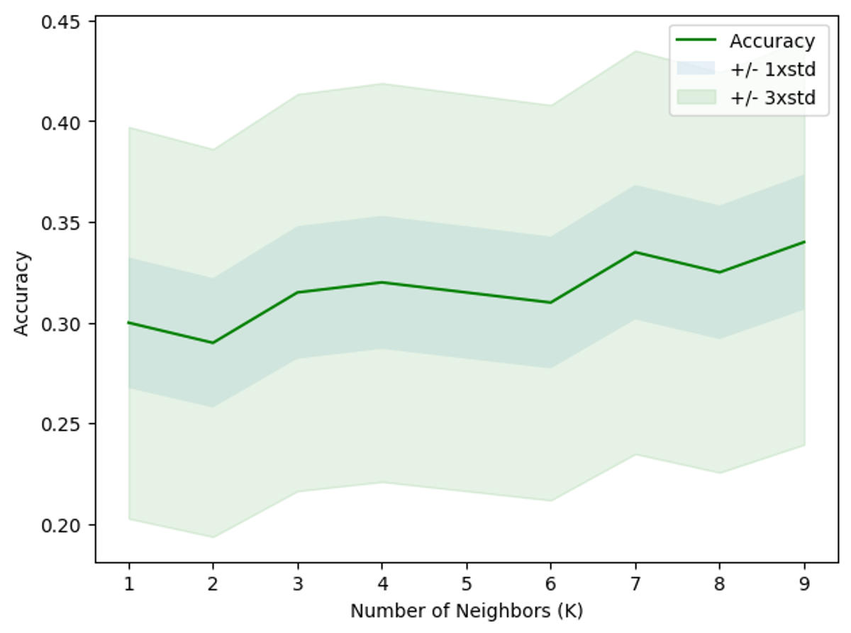
We can calculate the accuracy of KNN for different values of k.

Ks = 10
mean_acc = np.zeros((Ks-1))
std_acc = np.zeros((Ks-1))

for n in range(1,Ks):

    #Train Model and Predict
    neigh = KNeighborsClassifier(n_neighbors=n).fit(X_train,y_train)
    yhat=neigh.predict(X_test)
    mean_acc[n-1] = metrics.accuracy_score(y_test, yhat)

    std_acc[n-1]=np.std(yhat==y_test)/np.sqrt(yhat.shape[0])

mean_acc

array([0.3  , 0.29 , 0.315, 0.32 , 0.315, 0.31 , 0.335, 0.325, 0.34 ])

Plot the model accuracy for a different number of neighbors.

plt.plot(range(1,Ks),mean_acc,'g')
plt.fill_between(range(1,Ks),mean_acc - 1 * std_acc,mean_acc + 1 * std_acc, alpha=0.10)
plt.fill_between(range(1,Ks),mean_acc - 3 * std_acc,mean_acc + 3 * std_acc, alpha=0.10,color="green")
plt.legend(('Accuracy ', '+/- 1xstd','+/- 3xstd'))
plt.ylabel('Accuracy ')
plt.xlabel('Number of Neighbors (K)')
plt.tight_layout()
plt.show()

print( "The best accuracy was with", mean_acc.max(), "with k=", mean_acc.argmax()+1)

The best accuracy was with 0.34 with k= 9

Now let’s find the optimal k-value and the maximum accuracy

error_rate = []
for i in range(1,40):
 knn = KNeighborsClassifier(n_neighbors=i)
 knn.fit(X_train,y_train)
 pred_i = knn.predict(X_test)
 error_rate.append(np.mean(pred_i != y_test))
plt.figure(figsize=(10,6))
plt.plot(range(1,40),error_rate,color='blue', linestyle='dashed',
         marker='o',markerfacecolor='red', markersize=10)
plt.title('Error Rate vs. K Value')
plt.xlabel('K')
plt.ylabel('Error Rate')
print("Minimum error:-",min(error_rate),"at K =",error_rate.index(min(error_rate)))

Minimum error:- 0.59 at K = 37

Press enter or click to view image in full size

Conclusion

This article presents a comprehensive walkthrough of an end-to-end project using the K-Nearest Neighbors (KNN) algorithm in Python. The KNN algorithm is a supervised learning method used for classification by analyzing the ‘K’ nearest data points to predict the class of a given point. The article thoroughly explains the steps from loading the dataset, pre-processing data, selecting features, splitting data into training and testing sets, to training the KNN model with different values of ‘K’, and evaluating its performance.

Key points highlighted in the article include:

• Introduction to KNN: It describes the basics of the KNN algorithm, emphasizing its reliance on the proximity of data points to make predictions. It also discusses the challenge of choosing the optimal ‘K’ value, which significantly impacts model performance.
• Dataset Description: The article uses a dataset from a telecommunications provider, aiming to classify customers into four service usage categories based on demographic data. This real-world application underlines the practicality of KNN in classification problems.
• Data Preprocessing: This section covers data visualization, normalization, and splitting into training and testing sets, essential steps for preparing data for model training.
• Model Training and Prediction: It details the process of training the KNN model with the training data and making predictions on the test data. The article emphasizes the importance of experimenting with different ‘K’ values to find the optimal model performance.
• Evaluation of Model Performance: The article not only uses accuracy as a metric to evaluate model performance but also investigates error rates to determine the most appropriate ‘K’ value. The use of plots to visualize the relationship between ‘K’ and model accuracy/error provides a clear guide for selecting ‘K’.
• Optimal ‘K’ Value Selection: Through experimentation, it is demonstrated how different ‘K’ values affect the model’s accuracy, leading to the identification of the optimal ‘K’ value that minimizes error rates and maximizes prediction accuracy.

The conclusion of the article is that while there’s no one-size-fits-all method for selecting the ‘K’ value in KNN, a systematic approach involving trial and error, supported by visual aids like error rate plots, can effectively identify the optimal ‘K’. The article effectively illustrates the end-to-end process of applying KNN to a practical classification problem, providing readers with the knowledge to implement their own KNN models. It encourages experimentation with different ‘K’ values and underscores the significance of preprocessing and evaluating model performance to achieve the best results.

#I am happy to receive any feedback about this article;

#Please feel free to connect on linkedin;

#Please feel free to explore my portfolio on Github;

#In case you want to read more about my articles on medium, I would be very glad to meet with you as a follower;

I write about #Machine Learning, #Data Science, #Energy, #Renewable Energy, #Artificial Intelligence, #Project Management, #Strategy, #Business Analytics, #Statistics and Probability

### Thank you for !
#Saeed Aghabozorgi and IBM dataset