Understanding Unsupervised Learning with a Focus on KMeans Clustering in Real Data Application

Uncovering hidden patterns and structures in unlabelled data and a worldwide map view from a data science perspective

Introduction

Unsupervised learning is a type of machine learning where algorithms are trained on data without explicit instructions on what to do with it. In contrast to supervised learning, where models are trained on labeled data, unsupervised learning deals with data that has no labels or predefined categories.

The term “unsupervised” is derived from the absence of a supervising element (like labeled outcomes or specific instructions) guiding the learning process. Instead, the algorithms must discern patterns, structures, or features in the data autonomously. This independence from direct human oversight or explicit target outputs is what fundamentally characterizes unsupervised learning and gives it its name.

Although most of the applications of Machine Learning today are based on supervised learning, the vast majority of the available data is unlabeled: we have the input features X, but we do not have the labels y. This article aims to elucidate the concept of unsupervised learning and delve into one of its most prominent techniques: KMeans clustering using real-data.

Figure 1 nicely reveals the final result of the KMeans clustering in a 3D view and highlights in red X, which represents the centroid point for each cluster.

Enhancing KMeans with KMeans++: A Leap in Centroid Initialization

In KMeans, the initial placement of centroids can greatly influence the final clustering outcome. A poor choice of initial centroids can lead to suboptimal clustering, increased iterations, and even convergence to local minima. Recognizing this challenge, the KMeans algorithm in Scikit-Learn, by default, includes multiple runs (controlled by the n_init parameter, typically set to 10) with different random initializations, choosing the model with the lowest inertia (the mean squared distance between each instance and its closest centroid) as the best solution.

The introduction of KMeans++ has been a game-changer in the realm of KMeans clustering, addressing one of the algorithm’s fundamental challenges: the random initialization of centroids. KMeans++ presents a more intelligent way of initializing centroids that significantly reduces the chances of falling into suboptimal solutions. The steps are as follows:

1. Random Start: Select the first centroid (c(1)) randomly from the dataset.
2. Probabilistic Selection: For each subsequent centroid (c(i)), choose a new data point (x(i)) with a probability proportional to D(x(i))², where D(x(i)) is the distance between x(i) and the nearest centroid already chosen.
3. Repeat: Continue this process until all ‘k’ centroids are selected.

This method ensures that the initial centroids are spread out, making it more likely for KMeans to converge on an optimal solution.

This smarter initialization strategy not only enhances the quality of the clustering results but also makes the algorithm more robust and efficient. As data continues to grow in complexity, such advancements in algorithms like KMeans++ are pivotal in extracting more accurate and meaningful insights from the data.

The KMeans class in Scikit-Learn uses KMeans++ for initialization by default. If desired, one can revert to the original random initialization by setting the init parameter to "random". However, this is rarely necessary due to the effectiveness of the KMeans++ approach.

Real-Data and Step-by-Step Process

The data set is related to worldwide countries and its particularly information. The source comes from the US government. https://www.cia.gov/library/publications/the-world-factbook/docs/faqs.html

Exploratory Data Analysis

Let’s have a look at the data and create some visualizations.

df.info()
<class 'pandas.core.frame.DataFrame'>
RangeIndex: 227 entries, 0 to 226
Data columns (total 20 columns):
 #   Column                              Non-Null Count  Dtype
---  ------                              --------------  -----
 0   Country                             227 non-null    object
 1   Region                              227 non-null    object
 2   Population                          227 non-null    int64
 3   Area (sq. mi.)                      227 non-null    int64
 4   Pop. Density (per sq. mi.)          227 non-null    float64
 5   Coastline (coast/area ratio)        227 non-null    float64
 6   Net migration                       224 non-null    float64
 7   Infant mortality (per 1000 births)  224 non-null    float64
 8   GDP ($ per capita)                  226 non-null    float64
 9   Literacy (%)                        209 non-null    float64
 10  Phones (per 1000)                   223 non-null    float64
 11  Arable (%)                          225 non-null    float64
 12  Crops (%)                           225 non-null    float64
 13  Other (%)                           225 non-null    float64
 14  Climate                             205 non-null    float64
 15  Birthrate                           224 non-null    float64
 16  Deathrate                           223 non-null    float64
 17  Agriculture                         212 non-null    float64
 18  Industry                            211 non-null    float64
 19  Service                             212 non-null    float64
dtypes: float64(16), int64(2), object(2)
memory usage: 35.6+ KB

plt.figure(figsize=(10,6),dpi=200)
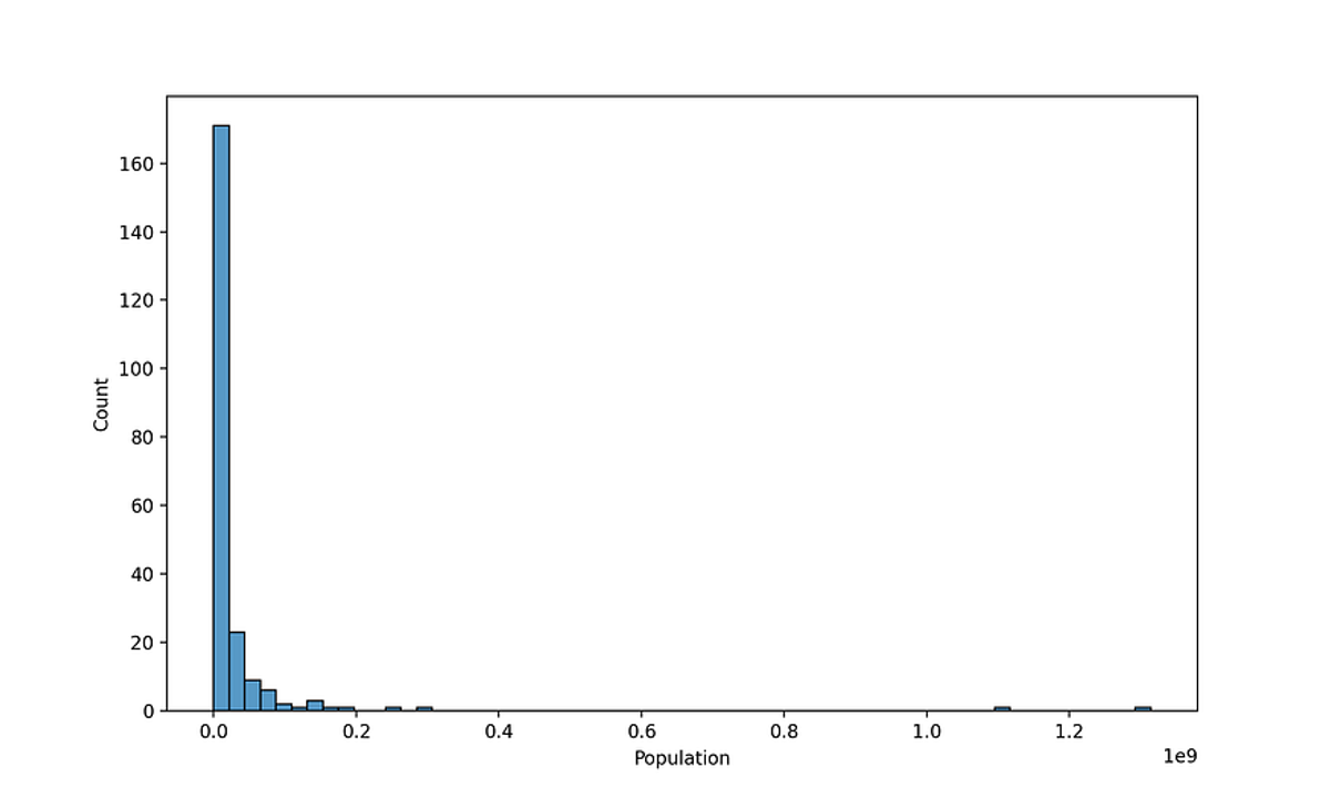
sns.histplot(data=df[df['Population']<1500000000],x='Population', bins=60)

Figure 2— Histogram showing the population size of the countries in the dataset

The histogram in Figure 2 depicts the distribution of population sizes in countries across the entiry world. The x-axis is scaled in scientific notation, indicating population size up to 1e9 (1.5 billion) — China and India are the ones larger than 1 billion. The histogram is heavily skewed to the left, with the first bins concentrated in population up to 200 million, showing the highest count by a significant margin. There are a few countries with population sizes ranging between 200 million to nearly 1 billion, but these are relatively rare compared to the first category.

plt.figure(figsize=(8, 6), dpi=200)
sns.barplot(data=df, y='GDP ($ per capita)', x='Region', hue='Region', estimator=np.mean, errorbar=('sd'))

# Rotating x-ticks
plt.xticks(rotation=90)

# Reducing the font size of x and y labels
plt.xlabel("Region", fontsize=9)
plt.ylabel("GDP ($ per capita)", fontsize=9)

# Optionally, adjust the tick labels font size
plt.tick_params(axis='x', labelsize=8)  # For x-axis
plt.tick_params(axis='y', labelsize=8)  # For y-axis

plt.tight_layout()

Press enter or click to view image in full size

Figure 3. Bar chart representing the mean GDP per capita for various regions around the world.

Figure 3 provides a bar chart representing the mean GDP per capita for various regions around the world. The bars indicate the average GDP value, while the vertical lines (error bars) represent the standard deviation, giving a sense of the variability or spread of GDP values within each region.

Here are some observations that can be made from the chart:

1. Regional Economic Disparities: There is a noticeable disparity in the GDP per capita across different regions. For instance, the region represented by the tallest green bar significantly outpaces others, suggesting a higher average GDP per capita.
2. Variability in GDP: The length of the error bars shows that some regions have a wide range in GDP per capita, indicating inequality within those regions. A region with a short error bar would have less variability in its GDP per capita, suggesting more uniform economic conditions.
3. Economic Comparisons: The bar chart facilitates direct comparisons between regions. For example, you can quickly discern which regions have higher or lower average GDP per capita and compare the degree of economic variation within each region.

Press enter or click to view image in full size

Figure 4. GDP per Region versus Literacy.

The scatter plot in Figure 4 shows the relationship between GDP per capita and literacy rates across different regions of the world. There appears to be a positive correlation between GDP per capita and literacy rates. This suggests that countries with higher GDP per capita tend to have higher literacy rates. Most of the data points are clustered towards the lower end of GDP per capita and span a wide range of literacy rates. There are fewer countries with very high GDP per capita, but those countries tend to have high literacy rates close to 100%.

• Western Europe and Northern America are represented by data points that are generally in the upper-right quadrant of the plot, indicating high GDP per capita and high literacy rates.
• Sub-Saharan Africa has many data points at the lower end of both GDP per capita and literacy rates.
• Asia (Ex. Near East) and Latin America & Caribbean have a wide spread across the GDP axis but are mostly in the middle to upper ranges of literacy rates.
• Eastern Europe, Oceania, and Baltics are more clustered, suggesting more uniformity in GDP and literacy rates within these regions.
• Near East and Northern Africa show a moderate level of both GDP and literacy rates with some variability.

There may be outliers or exceptions to these trends. For instance, there are countries with high GDP per capita but not the highest literacy rates or vice versa. This could be due to a variety of factors not captured by the plot, such as recent economic developments, natural resources, government policies on education, or cultural factors.

Always remember, while the scatter plot provides a visual correlation, it does not imply causation. There could be many underlying factors influencing the relationship between GDP and literacy rates that are not immediately apparent from the graph.

Press enter or click to view image in full size

Figure 5. Correlation Matrix.

The heatmap in Figure 5 illustrates the correlation matrix for various indicators of the dataset containing demographic, economic, and other attributes of different geographical entities (countries, regions, etc.)

Darker shades of blue indicate a strong positive correlation, while darker shades of green represent a strong negative correlation. Lighter colors or white suggest a weaker or no correlation.

High Positive Correlations:

• Birthrate and Infant mortality (0.85): This suggests that places with higher birthrates also tend to have higher infant mortality rates, which could be indicative of less developed healthcare systems.
• Phones (per 1000) and GDP ($ per capita) (0.83): This indicates that wealthier countries tend to have more phones per 1000 people, which could be related to better infrastructure and higher standards of living.
• Literacy (%) and Phones (per 1000) (0.60): This suggests that countries with higher literacy rates also have more widespread use of phones, possibly due to better education and access to technology.
• Service and GDP ($ per capita) (0.55): This indicates that countries with higher GDP per capita have a larger service sector, common in more developed economies.

High Negative Correlations:

• Birthrate and Literacy (%) (-0.79): This suggests that higher literacy rates often correspond with lower birthrates, which may be associated with better education and family planning.
• Infant mortality and GDP ($ per capita) (-0.67): This indicates that wealthier countries typically have lower infant mortality rates, likely due to better healthcare systems.

Notable Observations:

• Agriculture has a strong negative correlation with GDP ($ per capita) (-0.61), indicating that countries with higher GDPs have a smaller agricultural sector as a proportion of their economy, which is typical as economies develop and diversify.
• There are many correlations between indicators that are weak, suggesting no strong linear relationship.

The correlations between economic indicators (GDP, Phones, Service) and social indicators (Literacy, Infant mortality) are particularly strong, suggesting a close link between economic development and social outcomes. The correlations between demographic indicators (Birthrate, Deathrate, Infant mortality) are also significant, reflecting natural demographic trends.

I will repeat, it’s important to note that correlation does not imply causation. The relationships shown here indicate patterns and associations but do not necessarily indicate that one variable causes the other. Further analysis, such as regression modeling, causal inference and business knowledge, would be needed to understand the underlying mechanisms driving these correlations.

Data Engineering

Now let’s deal with missing data and prepar the dataset for modeling. Just follow the codes below:

df.isnull().sum()
Country                                0
Region                                 0
Population                             0
Area (sq. mi.)                         0
Pop. Density (per sq. mi.)             0
Coastline (coast/area ratio)           0
Net migration                          3
Infant mortality (per 1000 births)     3
GDP ($ per capita)                     1
Literacy (%)                          18
Phones (per 1000)                      4
Arable (%)                             2
Crops (%)                              2
Other (%)                              2
Climate                               22
Birthrate                              3
Deathrate                              4
Agriculture                           15
Industry                              16
Service                               15
dtype: int64

What countries have NaN for Agriculture? What is the main aspect of these countries? Noticed most of these countries are tiny islands, with the exception of Greenland and Western Sahara. It is acceptable to fill any of these countries missing NaN values with 0, since they are so small or essentially non-existant. There are 15 countries in total.

df[df['Agriculture'].isnull()]['Country']

3            American Samoa
4                   Andorra
78                Gibraltar
80                Greenland
83                     Guam
134                 Mayotte
140              Montserrat
144                   Nauru
153      N. Mariana Islands
171            Saint Helena
174    St Pierre & Miquelon
177              San Marino
208       Turks & Caicos Is
221       Wallis and Futuna
223          Western Sahara
Name: Country, dtype: object

#Filling Agriculture with 0

df[df['Agriculture'].isnull()] = df[df['Agriculture'].isnull()].fillna(0)

Notice that climate is missing for a few countries, but not the Region! Let’s use this to our advantage. Fill in the missing Climate values based on the mean climate value for its region. The same occur with Literacy missing. Let’s use the same tactic as we did with Climate missing values and fill in any missing Literacy values with the mean Literacy of the Region.

Finally, for simplicity let’s drop the other missing values for only a few countries and this last step will leave the dataset with zero missing values.

#Filling in the missing Climate values based on the mean Climate value for its region

df['Climate'] = df['Climate'].fillna(df.groupby('Region')['Climate'].transform('mean'))


#Filling in the missing Literacy values based on the mean Literacy value for its region

df['Literacy (%)'] = df['Literacy (%)'].fillna(df.groupby('Region')['Literacy (%)'].transform('mean'))

df.isnull().sum()

Country                               0
Region                                0
Population                            0
Area (sq. mi.)                        0
Pop. Density (per sq. mi.)            0
Coastline (coast/area ratio)          0
Net migration                         1
Infant mortality (per 1000 births)    1
GDP ($ per capita)                    0
Literacy (%)                          0
Phones (per 1000)                     2
Arable (%)                            1
Crops (%)                             1
Other (%)                             1
Climate                               0
Birthrate                             1
Deathrate                             2
Agriculture                           0
Industry                              1
Service                               1

#Dropping the remaining missing rows

df = df.dropna()

It is now time to prepare the data for clustering. The Country column is still a unique identifier string, so it won’t be useful for clustering, since its unique for each point. We will drop the column. We also need to create the X array of features, the Region column is still categorical strings, let’s use Pandas to create dummy variables from this column and finalize X matrix of continuous features along with the dummy variables for the Regions. The data ends up with a matrix of 221 rows by 29 columns and non-null information.

#Dropping Country column
X = df.drop("Country", axis=1)

#Creating dummy variables
X = pd.get_dummies(X)
X = X.astype(int)

X.info()

<class 'pandas.core.frame.DataFrame'>
Index: 221 entries, 0 to 226
Data columns (total 29 columns):
 #   Column                                      Non-Null Count  Dtype
---  ------                                      --------------  -----
 0   Population                                  221 non-null    int32
 1   Area (sq. mi.)                              221 non-null    int32
 2   Pop. Density (per sq. mi.)                  221 non-null    int32
 3   Coastline (coast/area ratio)                221 non-null    int32
 4   Net migration                               221 non-null    int32
 5   Infant mortality (per 1000 births)          221 non-null    int32
 6   GDP ($ per capita)                          221 non-null    int32
 7   Literacy (%)                                221 non-null    int32
 8   Phones (per 1000)                           221 non-null    int32
 9   Arable (%)                                  221 non-null    int32
 10  Crops (%)                                   221 non-null    int32
 11  Other (%)                                   221 non-null    int32
 12  Climate                                     221 non-null    int32
 13  Birthrate                                   221 non-null    int32
 14  Deathrate                                   221 non-null    int32
 15  Agriculture                                 221 non-null    int32
 16  Industry                                    221 non-null    int32
 17  Service                                     221 non-null    int32
 18  Region_ASIA (EX. NEAR EAST)                 221 non-null    int32
 19  Region_BALTICS                              221 non-null    int32
 20  Region_C.W. OF IND. STATES                  221 non-null    int32
 21  Region_EASTERN EUROPE                       221 non-null    int32
 22  Region_LATIN AMER. & CARIB                  221 non-null    int32
 23  Region_NEAR EAST                            221 non-null    int32
 24  Region_NORTHERN AFRICA                      221 non-null    int32
 25  Region_NORTHERN AMERICA                     221 non-null    int32
 26  Region_OCEANIA                              221 non-null    int32
 27  Region_SUB-SAHARAN AFRICA                   221 non-null    int32
 28  Region_WESTERN EUROPE                       221 non-null    int32
dtypes: int32(29)
memory usage: 26.8 KB

Due to some measurements being in terms of percentages and other metrics being total counts, such as Population, we should scale this data first. It is important to scale the input features before you run KMeans, or the clusters may be very stretched and KMeans will perform poorly. Scaling the features does not guarantee that all the clusters will be nice and spherical, but it generally improves results. With Sklearn we will scale the X feature. Follow a full explanation of the code:

• scaler = StandardScaler(): Here, an instance of the StandardScaler class is created and assigned to the variable scaler. This object will be used to perform the standardization.
• scaled_X = scaler.fit_transform(X):
• X: This represents your original dataset. It's assumed to be a 2D array (like a table), where rows are samples and columns are features.
• fit_transform: This method is a combination of two steps:
• fit: The fit method computes the mean and standard deviation for each feature in X. These calculated values are necessary for the subsequent scaling. Essentially, it's "learning" the parameters needed to scale the data.
• transform: The transform method then uses these learned parameters to standardize the data. Standardization is done by subtracting the mean and then dividing by the standard deviation for each feature. The formula is:
• z=(x−μ)/σ
• where x is the original feature value, μ is the mean of the feature, and σσ is the standard deviation of the feature.
• The fit_transform method is a convenient way to perform both steps in one call. It's often used in training data but should be used with caution to avoid data leakage in a machine learning pipeline.
• scaled_X: This is the result of the standardization process. It's a transformed version of X where each feature now has a mean of 0 and a standard deviation of 1. This standardization can improve the performance and convergence speed of many machine learning algorithms.

from sklearn.preprocessing import StandardScaler

scaler = StandardScaler()
scaled_X = scaler.fit_transform(X)

Standardization is particularly important for models that rely on the distance between data points, like KMeans clustering or principal component analysis (PCA). It ensures that each feature contributes equally to the distance computations and that the model isn’t unfairly influenced by features on larger scales.

Creating and Fitting KMeans Model

Curiously there is no universal definition of what a cluster is: it really depends on the context, and different algorithms will capture different kinds of clusters. Some algorithms look for instances centered around a particular point, called a centroid. Others look for continuous regions of densely packed instances: these clusters can take on any shape. Some algorithms are hierarchical, looking for clusters of clusters. And the list goes on.

The computational complexity of the algorithm is generally linear with regard to the number of instances m, the number of clusters k, and the number of dimensions n. However, this is only true when the data has a clustering structure. If it does not, then in the worst-case scenario the complexity can increase exponentially with the number of instances. In practice, this rarely happens, and KMeans is generally one of the fastest clustering algorithms.

The aim of our KMeans algorithm implemented is to partition a set of data points into K clusters, where each data point belongs to the cluster with the nearest mean. Here’s how we generally code about creating and fitting a K-means model; i) Use a lop to generate and fit multiple Kmeans models, testing several clusters. ii) implement and test several cluster; in our project we are going to test from 2 to 30 clusters in order to optimize coding and later on evaluate the best model.

In the context of KMeans, inertia is the sum of squared distances of samples to their closest cluster center and it’s one way to explore to right number of finding clusters. It’s a measure of how internally coherent clusters are. The goal of this code is to compute the inertia for different numbers of clusters and store these values. By plotting these inertia values against the number of clusters, it is possible to inspect the “elbow” point, where the rate of decrease of inertia with respect to the number of clusters becomes significantly slower. This point is considered a good estimate for the optimal number of clusters.

from sklearn.cluster import KMeans

#Looping for plotting the Inertia computation
ssd = []

for k in range(2,30):

    model = KMeans(n_clusters = k)

    model.fit(scaled_X)

    ssd.append(model.inertia_);

To find the elbow point, typically a plot is created using libraries like matplotlib or seaborn with the number of clusters on the x-axis and the corresponding inertia values on the y-axis. The “elbow” in this plot indicates the most appropriate number of clusters for your dataset. This is a heuristic method and involves a bit of subjectivity, as the elbow might not always be sharply defined.

plt.figure(figsize=(5,5), dpi=200)
plt.plot(range(2,30), ssd, "o--")
plt.xlabel("k Value")
plt.ylabel("Sum of Squared Distances")
plt.tight_layout

Press enter or click to view image in full size

Figure 6. K Value versus Inertia .

The plot in Figure 6 shows the “Elbow” Method analysis used to determine the optimal number of clusters for KMeans clustering. This graph is plotting the inertia, which is the sum of squared distances of samples, to their closest cluster center for different values of k, which is the number of clusters.

The inertia decreases rapidly as the number of clusters increases from 2 and starts to level off around k=10, suggesting that the rate of decrease is slowing down. After this point, the curve becomes more gradual. This suggests that the optimal number of clusters for the dataset might be around 10 since adding more clusters beyond this point does not reduce the inertia by a significant margin.

Nevertheless, choosing the number of clusters is still somewhat subjective because the plot does not have a sharp, well-defined “elbow”. A domain expert might also consider other factors related to the specific context of the data to decide on the most appropriate number of clusters.

I consider the Inertia technique for choosing the best value for the number of clusters coarse. A more precise approach, and more computationally expensive, is to use the silhouette score, which is the mean silhouette coefficient over all the instances. An instance’s silhouette coefficient is equal to (b — a) / max(a, b), where a is the mean distance to the other instances in the same cluster (i.e., the mean intra-cluster distance) and b is the mean nearest-cluster distance (i.e., the mean distance to the instances of the next closest cluster, defined as the one that minimizes b, excluding the instance’s own cluster). The silhouette coefficient can vary between –1 and +1. A coefficient close to +1 means that the instance is well inside its own cluster and far from other clusters, while a coefficient close to 0 means that it is close to a cluster boundary. Finally, a coefficient close to –1 means that the instance may have been assigned to the wrong cluster. Let’s compare the silhouette scores for different numbers of clusters (see Figure 6).

To compute the silhouette score, we use Scikit-Learn’s silhouette_score() function, giving it all the instances in the dataset and the labels they were assigned.

from sklearn.metrics import silhouette_score

silhouette_score(X, KMeans.labels_)

# Assuming X is our data

# Define the range of k
k_values = range(2, 9)

# Fit KMeans models for each k and store them
kmeans_per_k = [KMeans(n_clusters=k, random_state=42).fit(X) for k in k_values]

# Compute Silhouette Scores
silhouette_scores = [silhouette_score(X, model.labels_) for model in kmeans_per_k]

# Plotting the silhouette scores
plt.figure(figsize=(8, 3))
plt.plot(k_values, silhouette_scores, "bo-")
plt.xlabel("$kquot;)
plt.ylabel("Silhouette score")
plt.grid()
plt.show()

Press enter or click to view image in full size

Figure 7. Selecting the number of clusters k using the silhouette score plot.

As you can see, this visualization in Figure 7 is much richer than the previous one. It seems that the best choice is k = 2 and it also underlines the fact that k = 3 is quite good as well, besides both are better than k from 4 to 9. This was not visible when comparing inertia. In general, there is no single rule that will reliably guide how many clusters to claim and no reasonable 100% correct answer. That’s why is so important to have a insightful business knowledge about the subject being explored. Many times we need to trust on our business acumem to decide the best k. In this project we decided to proceed with k = 3.

The provided code below is using the KMeans clustering algorithm from a machine learning library scikit-learn. Let’s break down each part of the code for a clearer understanding:

model = KMeans(n_clusters=3):

• This line creates an instance of the KMeans class.
• KMeans is ther unsupervised machine learning algorithm used for clustering.
• n_clusters=3 specifies that the algorithm should try to find 3 clusters in the data. This is a parameter that needs to be defined; the choice of how many clusters to use can significantly impact the results and often depends on the specific use case or domain knowledge.

model.fit(scaled_X):

• This line applies the KMeans algorithm to the data stored in scaled_X.
• scaled_X is the dataset that has been scaled or normalized. If the features are on different scales, one feature might disproportionately influence the cluster assignments.
• The fit method computes the centroids of the clusters (which are the mean of the points in each cluster) and assigns each data point in scaled_X to one of the clusters.

#Create a cluster labels and model for a chosen solution of k = 3

model = KMeans(n_clusters=3)

model.fit(scaled_X)

Geographical Model Intepretation

Now it’s time to interpret this model through visualizing the clusters countries on a map and give a real world solution to this data science project. Let’s plot the clusters on a country level choropleth map and interpret the results.

iso_mapping = iso_codes.set_index('Country')['ISO Code'].to_dict()

df.loc[:, 'ISO Code'] = df['Country'].map(iso_mapping)

df.loc[:, 'Cluster'] = model.labels_

import plotly.express as px

#Plotting the clusters

fig = px.choropleth(df, locations="ISO Code",
                   color = "Cluster",
                   hover_name = "Country",
                   color_continuous_scale = "Turbo")

fig.show()

Press enter or click to view image in full size

Figure 8. Global view according to KMeans solution equal 3.

The map assembled in Figure 8 communicates a global view with countries color-coded according to which of three clusters they belong to, in conformity to the result of the KMeans clustering. The colors correspond to the three different clusters with a color bar on the right indicating the cluster assignment for each country.

• The bottom of the bar represents Cluster 0.
• The middle of the bar represents Cluster 1.
• The top of the bar represents Cluster 2.
• The countries in green representing Cluster 0. This cluster seems to include countries from North and South America, parts of Europe, and a few other scattered countries.
• The countries in red represent Cluster 1, which appears to predominantly include countries from Africa and the Middle East, with some in Europe and Asia.
• The countries in purple correspond to Cluster 2, which seems to consist mainly of countries from Asia and Oceania, with some in Europe.

The clustering result implies that countries within the same color share similar characteristics in the dataset used for the KMeans algorithm. It is clearly based on different levels of economic development, health statistics, geographic and environmental data, similar climates, topographies, natural resources, etc.

Conclusion

The article provides an insightful exploration into the realm of unsupervised machine learning, emphasizing the KMeans clustering algorithm. It elucidates how KMeans, particularly with the KMeans++ initialization, effectively uncovers hidden patterns in unlabelled data, a common scenario given the abundance of unlabeled datasets in various domains.

The application of KMeans to a real-world dataset of worldwide countries, drawn from the US government’s database, showcases the algorithm’s practical utility. The exploratory data analysis, involving visualizations of population distributions, GDP per capita, literacy rates, and other significant factors, sets the stage for understanding the dataset’s intrinsic characteristics. The correlation matrix, revealing intricate relationships between various socio-economic indicators, further enriches this understanding.

The article meticulously guides us through the data engineering steps, addressing missing data and preparing the dataset for modeling. The process of standardizing the data underscores the importance of feature scaling in clustering algorithms. The subsequent creation and fitting of the KMeans model, along with the use of the “elbow” method and silhouette scores for determining the optimal number of clusters, demonstrate a comprehensive approach to applying KMeans in a real-world scenario.

The geographical interpretation of the model, visualizing the clusters of countries on a map, is particularly striking. It reveals how countries within the same cluster share similarities in various dimensions like economic status, health indicators, and geographic attributes. This visual representation not only validates the KMeans algorithm’s efficacy but also provides a tangible, real-world application of unsupervised learning.

In conclusion, the article serves as an exemplary guide in demystifying unsupervised learning, particularly KMeans clustering. It skillfully bridges the gap between theoretical concepts and practical application, offering valuable insights for both novice and experienced practitioners in the field of data science. The integration of real-world data with sophisticated analytical techniques exemplifies the power of machine learning in uncovering hidden patterns and facilitating informed decision-making based on comprehensive data analysis.

#I am happy to receive any feedback about this article;

#Please feel free to connect on linkedin;

#Please feel free to explore my portfolio on Github;

#In case you want to read more about my articles on medium, I would be very glad to meet with you as a follower;

I write about #Machine Learning, #Data Science, #Energy, #Renewable Energy, #Artificial Intelligence, #Project Management, #Strategy, #Business Analytics, #Statistics and Probability